본 포스트에서는 Model-Agnostic Method중 하나인 Partial Dependence Plot(PDP)를 이용하여 이전 챕터에서 iris 데이터를 학습한 Neural Network 에 적용해보도록 하겠습니다.
Partial Dependence Plot(PDP) 설명
Partial Dependence Plot(PDP)는 Model-Agnostic Method 중 하나로 학습된 모델을 가지고 데이터셋을 특정 feature들을 변환하면서 바뀌는 모델 출력값들의 평균을 가지고 모델을 해석하는 방법입니다.
예를 들어 iris 데이터를 가지고 학습한 모델에 iris데이터의 모든 instance에 대해 꽃받침의 길이를 최솟값부터 최댓값까지 변환하면서 바뀌는 모델의 softmax 값의 평균을 가지고 모델을 해석합니다.
해당 수식은 다음과 같습니다.
그러면 이제 iris 데이터와 학습된 모델을 가지고 PDP를 그려보도록 하겠습니다.
필요 라이브러리 import
import tensorflow as tf
import numpy as np
import matplotlib.pyplot as plt
%matplotlib inline
from sklearn.datasets import load_iris
pdp를 그리기 위해 필요한 라이브러리들을 import 합니다.
iris 데이터, 학습한 모델 불러오기
 iris_dataset = load_iris()
 model = tf.keras.models.load_model('iris_model.h5')

 target_names = iris_dataset['target_names']
 feature_names = iris_dataset['feature_names']
iris 데이터와 이 전 챕터에서 학습한 모델을 불러옵니다.
자주 사용할 target_names와 feature_names를 따로 변수로 만들어 줍니다.
Partial Dependence Plot(PDP) 그리기
plt.figure(figsize=(10,10))
color_list = ['r-', 'g-', 'b-']
plt_term = 100

for feature_idx in range(len(feature_names)):
    tmp_data = np.copy(iris_dataset['data'])
    index = np.linspace(min(tmp_data[:, feature_idx]), max(tmp_data[:, feature_idx]), plt_term)
    results = []
    for i in index:
        tmp_data[:, feature_idx] = i
        result = model.predict(tmp_data)
        f_hat = np.mean(result, axis=0)
        results += [f_hat]

    results = np.array(results)
    plt.subplot(2,2,feature_idx+1)
    plt.xlabel(feature_names[feature_idx])

    for target_idx in range(len(target_names)):
        plt.plot(index, results[:,target_idx], color_list[target_idx], label=target_names[target_idx])

    plt.legend()
    plt.ylim(0,1)
PDP를 그리는 코드는 위와 같습니다. 각 feature를 돌면서 각 feature의 최솟값 부터 최댓값 까지 값을 변환하면서 모델의 softmax 값들의 target에 대한 평균 값을 수집합니다. 수집한 데이터를 가지고 setosa는 빨간선, versicolor는 초록선, virginica는 파란선으로 표시합니다.
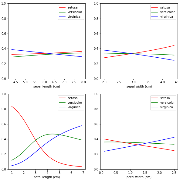
PDP 결과를 살펴보면 다른 feature들에 대해서는 softmax 값들이 비슷하나 꽃잎의 길이에 대해서는 차이가 많이 나는 것을 볼 수 있습니다. 위 결과에 따르면 모델은 길이가 짧아질수록 setosa라고 예측하는 경향이 있다는 것을 알 수 있습니다.
그리고 결과를 전체적으로 보았을 때는 모델은 꽃받침의 길이가 짧고, 너비가 좁고, 꽃잎의 길이가 길고, 너비가 크면 virginica라고 예측하는 경향이 있다는 것을 알 수 있습니다.
PDP 2D 그리기
 plt.figure(figsize=(15,30))
 color_map = ['Reds', 'Greens', 'Blues']
 plt_term = 30

for feature_idx_1 in range(len(feature_names)):
    for feature_idx_2 in range(feature_idx_1+1, len(feature_names)):
        tmp_data = np.copy(iris_dataset['data'])
        index_1 = np.linspace(min(tmp_data[:, feature_idx_1]), max(tmp_data[:, feature_idx_1]), plt_term)
        index_2 = np.linspace(min(tmp_data[:, feature_idx_2]), max(tmp_data[:, feature_idx_2]), plt_term)

        results_matrix = []
        for i_1 in index_1:
            tmp_data[:, feature_idx_1] = i_1
            results = []
            for i_2 in index_2:
                tmp_data[:, feature_idx_2] = i_2
                result = model.predict(tmp_data)
                f_hat = np.mean(result, axis=0)
                results += [f_hat]
            results_matrix = np.c_[results_matrix, results] if len(results_matrix) else results
        for target_idx in range(len(target_names)):
            ffeature_idx_1 = -1 if feature_idx_1 == 0 else feature_idx_1
            plt.subplot(6,3, 3*(ffeature_idx_1+feature_idx_2) + target_idx + 1)
            plt.xlabel(feature_names[feature_idx_1])
            plt.ylabel(feature_names[feature_idx_2])
            plt.title(target_names[target_idx])
            plt.imshow(results_matrix[::-1, [3*n +target_idx for n in range(plt_term)]], cmap=color_map[target_idx])
            plt.clim(0,1)
            plt.xticks(np.linspace(0,plt_term,10),labels=[round(index_1[plt_term*i//10],1) for i in range(10)])
            plt.yticks(np.linspace(plt_term,0,10),labels=[round(index_2[plt_term*i//10],1) for i in range(10)])
            plt.colorbar()
PDP 2D를 그리는 코드는 위와 같습니다. PDP 2D를 그리기 위해서는 4개의 feature들 중 2개씩 골라서 최솟값부터 최댓값까지 값을 변환하면서 모델의 softmax값을 가시화합니다. plot 하나에 3 target의 softmax를 담을 수 없으므로 target 별로 plot을 만들었고 표시 색깔은 이전과 동일하게 유지하였습니다.
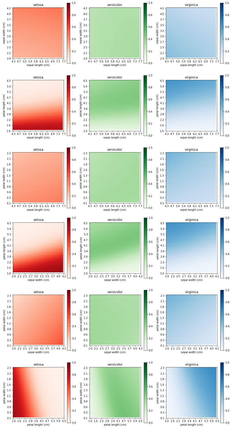
PDP 2D 결과를 살펴보면 다른 PDP 1D와 비슷하게 꽃받침에 길이에 대해서 모델의 setosa에 대한 softmax 값이 보다 민감하게 반응하는 것을 알 수 있습니다.